Edit this page
Open and issue
Logistic Regression
For this section we will work with the Titanic Data Set from Kaggle. We'll be trying to predict a classification problem - survival or deceased. Let's begin our understanding of implementing Logistic Regression in Python for classification. We'll use a "semi-cleaned" version of the titanic data set, if you use the data set hosted directly on Kaggle, you may need to do some additional cleaning not shown in this notebook.
Let's import some libraries and load the dataset:
import pandas as pd
import numpy as np
import matplotlib.pyplot as plt
import seaborn as sns
%matplotlib inline

train = pd.read_csv('../data/titanic_train.csv')
Let's view the data present in the dataset:
train.head()
| PassengerId | Survived | Pclass | Name | Sex | Age | SibSp | Parch | Ticket | Fare | Cabin | Embarked | |
| 0 | 1 | 0 | 3 | Braund, Mr. Owen Harris | male | 22.0 | 1 | 0 | A/5 21171 | 7.2500 | NaN | S |
| 1 | 2 | 1 | 1 | Cumings, Mrs. John Bradley (Florence Briggs Th... | female | 38.0 | 1 | 0 | PC 17599 | 71.2833 | C85 | C |
| 2 | 3 | 1 | 3 | Heikkinen, Miss. Laina | female | 26.0 | 0 | 0 | STON/O2. 3101282 | 7.9250 | NaN | S |
| 3 | 4 | 1 | 1 | Futrelle, Mrs. Jacques Heath (Lily May Peel) | female | 35.0 | 1 | 0 | 113803 | 53.1000 | C123 | S |
| 4 | 5 | 0 | 3 | Allen, Mr. William Henry | male | 35.0 | 0 | 0 | 373450 | 8.0500 | NaN | S |
Exploratory Data Analysis
Let's begin some exploratory data analysis! We'll start by checking out missing data!
Missing Data
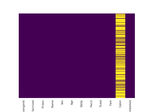
We can use seaborn to create a simple heatmap to see where we are missing data!
sns.heatmap(train.isnull(),yticklabels=False,cbar=False,cmap='viridis');
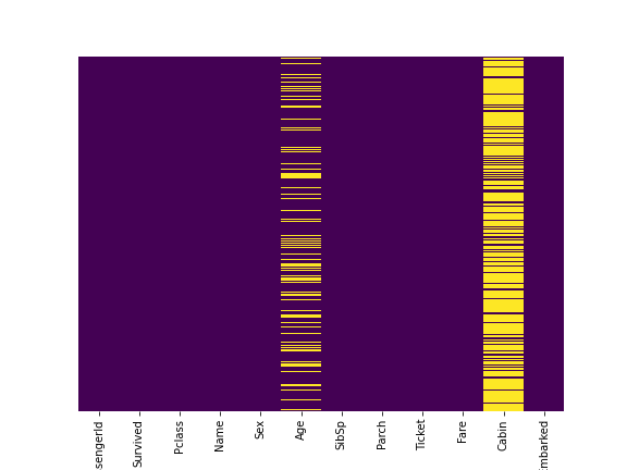
Roughly 20 percent of the Age data is missing. The proportion of Age missing is likely small enough for reasonable replacement with some form of imputation. Looking at the Cabin column, it looks like we are just missing too much of that data to do something useful with at a basic level. We'll probably drop this later, or change it to another feature like "Cabin Known: 1 or 0"
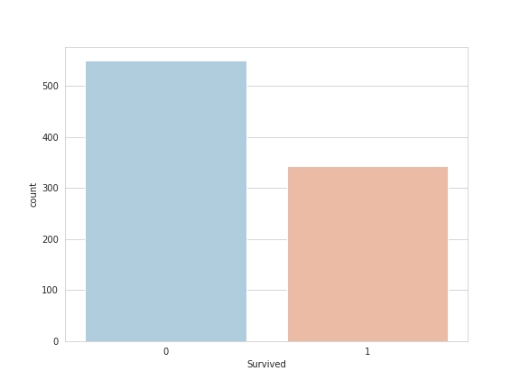
Let's continue on by visualizing some more of the data such as our target variable survival:
sns.set_style('whitegrid');
sns.countplot(x='Survived',data=train,palette='RdBu_r');
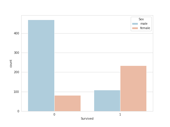
We can manipulate the data a bit and look at the difference in survival betwen men and women:
sns.set_style('whitegrid');
sns.countplot(x='Survived',hue='Sex',data=train,palette='RdBu_r');
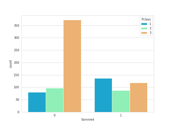
We can also split the data up based on the class level of the passengers:
sns.set_style('whitegrid');
sns.countplot(x='Survived',hue='Pclass',data=train,palette='rainbow');
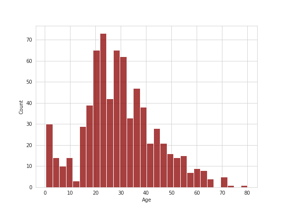
Let's now look at the distribution of age for the passengers:
sns.distplot(train['Age'].dropna(),kde=False,color='darkred',bins=30);
Data Cleaning
We want to fill in missing age data instead of just dropping the missing age data rows. One way to do this is by filling in the mean age of all the passengers (imputation). However we can be smarter about this and check the average age by passenger class. For example:
plt.figure(figsize=(12, 7));
sns.boxplot(x='Pclass',y='Age',data=train,palette='winter');
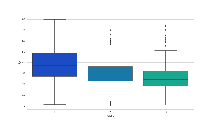
We can see the wealthier passengers in the higher classes tend to be older, which makes sense. We'll use these average age values to impute based on Pclass for Age.
def impute_age(cols):
    Age = cols[0]
    Pclass = cols[1]

    if pd.isnull(Age):
        if Pclass == 1:
            return 37
        elif Pclass == 2:
            return 29
        else:
            return 24
    else:
        return Age
Now apply that function:
train['Age'] = train[['Age','Pclass']].apply(impute_age,axis=1)
Now let's check that heat map again!
sns.heatmap(train.isnull(),yticklabels=False,cbar=False,cmap='viridis');
Great! Let's go ahead and drop the Cabin column and the row in Embarked that is NaN.
train.drop('Cabin',axis=1,inplace=True);
train.dropna(inplace=True);

train.head()
| PassengerId | Survived | Pclass | Name | Sex | Age | SibSp | Parch | Ticket | Fare | Embarked | |
| 0 | 1 | 0 | 3 | Braund, Mr. Owen Harris | male | 22.0 | 1 | 0 | A/5 21171 | 7.2500 | S |
| 1 | 2 | 1 | 1 | Cumings, Mrs. John Bradley (Florence Briggs Th... | female | 38.0 | 1 | 0 | PC 17599 | 71.2833 | C |
| 2 | 3 | 1 | 3 | Heikkinen, Miss. Laina | female | 26.0 | 0 | 0 | STON/O2. 3101282 | 7.9250 | S |
| 3 | 4 | 1 | 1 | Futrelle, Mrs. Jacques Heath (Lily May Peel) | female | 35.0 | 1 | 0 | 113803 | 53.1000 | S |
| 4 | 5 | 0 | 3 | Allen, Mr. William Henry | male | 35.0 | 0 | 0 | 373450 | 8.0500 | S |
Converting Categorical Features
We'll need to convert categorical features to dummy variables using pandas. If we do not convert then our machine learning algorithm won't be able to directly take in those features as inputs.
train.info()
<class 'pandas.core.frame.DataFrame'>
Int64Index: 889 entries, 0 to 890
Data columns (total 11 columns):
PassengerId    889 non-null int64
Survived       889 non-null int64
Pclass         889 non-null int64
Name           889 non-null object
Sex            889 non-null object
Age            889 non-null float64
SibSp          889 non-null int64
Parch          889 non-null int64
Ticket         889 non-null object
Fare           889 non-null float64
Embarked       889 non-null object
dtypes: float64(2), int64(5), object(4)
memory usage: 83.3+ KB
sex = pd.get_dummies(train['Sex'],drop_first=True)
embark = pd.get_dummies(train['Embarked'],drop_first=True)
train.drop(['Sex','Embarked','Name','Ticket'],axis=1,inplace=True)
train = pd.concat([train,sex,embark],axis=1)
train.head()
| PassengerId | Survived | Pclass | Age | SibSp | Parch | Fare | male | Q | S | |
| 0 | 1 | 0 | 3 | 22.0 | 1 | 0 | 7.2500 | 1 | 0 | 1 |
| 1 | 2 | 1 | 1 | 38.0 | 1 | 0 | 71.2833 | 0 | 0 | 0 |
| 2 | 3 | 1 | 3 | 26.0 | 0 | 0 | 7.9250 | 0 | 0 | 1 |
| 3 | 4 | 1 | 1 | 35.0 | 1 | 0 | 53.1000 | 0 | 0 | 1 |
| 4 | 5 | 0 | 3 | 35.0 | 0 | 0 | 8.0500 | 1 | 0 | 1 |
Great! Our data is ready for our model!
Building a Logistic Regression model
Let's start by splitting our data into a training set and test set (there is another test.csv file that you can play around with in case you want to use all this data for training).
Train Test Split
from sklearn.model_selection import train_test_split

X_train, X_test, y_train, y_test = train_test_split(train.drop('Survived',axis=1),
                                                    train['Survived'], test_size=0.30,
                                                    random_state=101)
Training and Predicting
from sklearn.linear_model import LogisticRegression

logmodel = LogisticRegression()
logmodel.fit(X_train,y_train)
predictions = logmodel.predict(X_test)
Let's move on to evaluate our model!
Evaluation
We can check precision,recall,f1-score using classification report!
from sklearn.metrics import classification_report

print(classification_report(y_test,predictions))
Not so bad! You might want to explore other feature engineering and the other titanic_text.csv file, some suggestions for feature engineering:
- Try grabbing the Title (Dr.,Mr.,Mrs,etc..) from the name as a feature
- Maybe the Cabin letter could be a feature
- Is there any info you can get from the ticket?