Linear Regression

The linear regression (LR) model is a simple machine learning approach used for target variables that are continuous (i.e. variables that are real-valued). The LR model takes as its input both a vector of features (conventionally labeled X) and a vector of labels (y). Often different terminology is used —calling X our set of variables or predictors, and y our outcome or dependent variable—but the idea is the same. The data are plotted, and a straight line is then fit to these data points. The objective is to fit the line to the data points so that the distance between the line and points are minimized.

Let's return to our running house price-prediction example. Predicting sales price from the features is a regression problem, because sale price varies continuously. What we're trying to find is some optimal function that, given a matrix of feature scores, can produce a set of continuous values that best approximates (for whatever definition of "best" we like) the true house price of our houses.

First we import the required libraries then investigate the data:

import pandas as pd
import numpy as np
import matplotlib.pyplot as plt
import seaborn as sns
%matplotlib inline

all_data = pd.read_csv('../data/house_prices.csv', sep=',', index_col=0).reset_index(drop=True)

all_data.info()

<class 'pandas.core.frame.DataFrame'>
RangeIndex: 1460 entries, 0 to 1459
Data columns (total 80 columns):
MSSubClass       1460 non-null int64
MSZoning         1460 non-null object
LotFrontage      1201 non-null float64
LotArea          1460 non-null int64
Street           1460 non-null object
Alley            91 non-null object
LotShape         1460 non-null object
LandContour      1460 non-null object
Utilities        1460 non-null object
LotConfig        1460 non-null object
LandSlope        1460 non-null object
Neighborhood     1460 non-null object
Condition1       1460 non-null object
Condition2       1460 non-null object
BldgType         1460 non-null object
HouseStyle       1460 non-null object
OverallQual      1460 non-null int64
OverallCond      1460 non-null int64
YearBuilt        1460 non-null int64
YearRemodAdd     1460 non-null int64
RoofStyle        1460 non-null object
RoofMatl         1460 non-null object
Exterior1st      1460 non-null object
Exterior2nd      1460 non-null object
MasVnrType       1452 non-null object
MasVnrArea       1452 non-null float64
ExterQual        1460 non-null object
ExterCond        1460 non-null object
Foundation       1460 non-null object
BsmtQual         1423 non-null object
BsmtCond         1423 non-null object
BsmtExposure     1422 non-null object
BsmtFinType1     1423 non-null object
BsmtFinSF1       1460 non-null int64
BsmtFinType2     1422 non-null object
BsmtFinSF2       1460 non-null int64
BsmtUnfSF        1460 non-null int64
TotalBsmtSF      1460 non-null int64
Heating          1460 non-null object
HeatingQC        1460 non-null object
CentralAir       1460 non-null object
Electrical       1459 non-null object
1stFlrSF         1460 non-null int64
2ndFlrSF         1460 non-null int64
LowQualFinSF     1460 non-null int64
GrLivArea        1460 non-null int64
BsmtFullBath     1460 non-null int64
BsmtHalfBath     1460 non-null int64
FullBath         1460 non-null int64
HalfBath         1460 non-null int64
BedroomAbvGr     1460 non-null int64
KitchenAbvGr     1460 non-null int64
KitchenQual      1460 non-null object
TotRmsAbvGrd     1460 non-null int64
Functional       1460 non-null object
Fireplaces       1460 non-null int64
FireplaceQu      770 non-null object
GarageType       1379 non-null object
GarageYrBlt      1379 non-null float64
GarageFinish     1379 non-null object
GarageCars       1460 non-null int64
GarageArea       1460 non-null int64
GarageQual       1379 non-null object
GarageCond       1379 non-null object
PavedDrive       1460 non-null object
WoodDeckSF       1460 non-null int64
OpenPorchSF      1460 non-null int64
EnclosedPorch    1460 non-null int64
3SsnPorch        1460 non-null int64
ScreenPorch      1460 non-null int64
PoolArea         1460 non-null int64
PoolQC           7 non-null object
Fence            281 non-null object
MiscFeature      54 non-null object
MiscVal          1460 non-null int64
MoSold           1460 non-null int64
YrSold           1460 non-null int64
SaleType         1460 non-null object
SaleCondition    1460 non-null object
SalePrice        1460 non-null int64
dtypes: float64(3), int64(34), object(43)
memory usage: 912.6+ KB

# Select only columns that are numeric
all_data = all_data.select_dtypes(['number'])

# Remove any rows that contain NaN
for ifeature in list(all_data):
    all_data = all_data[pd.notnull(all_data[ifeature])]

all_data.shape

(1121, 37)

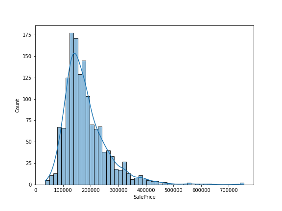
Let's also plot our target variable, Sales Price, to see what the distribution looks like:

sns.histplot(all_data['SalePrice'], kde=True)

Training a Linear Regression Model

We will need to first split up our data into an X array that contains the features to train on, and a y array with the target variable, in this case the Sale Price. We start by setting the X and y variables, split into train and test sets using the train_test_split function from scikit-learn and initialize the LinearRegression estimator:

from sklearn.model_selection import train_test_split

# Set input features and output variable
y = all_data['SalePrice']
X = all_data.drop(['SalePrice'], axis =1)

# Split data into test and train sets
X_train, X_test, y_train, y_test = train_test_split(X, y.to_numpy().ravel(), test_size=0.30, random_state=101)

# OLS (and many other variants of regression) is housed in the linear_model module
from sklearn.linear_model import LinearRegression

# initialize the model
lr_model = LinearRegression()

The LinearRegression estimator, unlike many others, has very few configurable parameters. Above, we initialize it with all of the default values by passing no arguments to the function. Now we're ready to fit some data! We can do that by calling the .fit() method. This will be true for every Estimator in scikit-learn. We will use our training sub-datasets we created:

# Fit the model
lr_model.fit(X_train, y_train);

Now we have a fitted model we need to evaluate the accuracy of this training process. We always want to evaluate the trained model prior to applying it to test data.

# The sklearn convention is to denote fitted parameters with a trailing underscore
print('Model y intercept:',lr_model.intercept_,'\n')
print('Model feature coefficients:',lr_model.coef_,'\n')

Model y intercept: -1348228.3926262031

Model feature coefficients: [-8.75772924e+01  5.95600326e+01  1.18930737e+00  1.38647884e+04
  4.91899261e+03  4.10628404e+02  1.81486446e+02  1.51819223e+01
  2.69056767e+01 -1.07411164e+00 -3.69107465e-01  2.54624576e+01
  1.84098928e+01  2.14677482e+01  7.35941390e+00  4.72370548e+01
 -8.14206679e+02 -6.09318362e+03 -1.52754837e+03 -1.82409326e+03
 -1.58292462e+04 -2.59304669e+04  5.44696494e+03 -4.36801780e+01
 -4.51893373e+01  4.11495671e+03  2.38219900e+01  4.82163185e+00
  2.38325092e+01  3.04386635e+01  9.87034508e+00  4.14229568e+01
  1.26489368e+02 -2.30107736e+00  2.62862323e+02  1.01150684e+02]

We can use these parameter estimates (y intercept and coefficients) to manually construct and apply a prediction equation (i.e., \(\hat{y} = -0.557 + 1.43x\)) if we want to. The other thing we can look at is the coefficient.

coeff_df = pd.DataFrame(lr_model.coef_,X.columns,columns=['Coefficient'])
coeff_df.head()

	Coefficient
MSSubClass	-87.577292
LotFrontage	59.560033
LotArea	1.189307
OverallQual	13864.788358
OverallCond	4918.992610

Interpreting the coefficients:

• Holding all other features fixed, a 1 unit increase in Lot Frontage is associated with an **increase of $59.56 **.
• Holding all other features fixed, a 1 unit increase in Lot Area is associated with an **increase of $1.18 **.
• Holding all other features fixed, a 1 unit increase in Overall Condition is associated with an **increase of $4918.99 **.

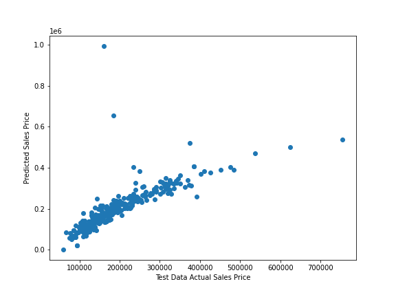
The next step is to use the trained model to predict new house Sale Price on new data. We do this by making use of the .predict() method that all Estimator classes implement. For example, here are the predicted scores for our X test data:

lr_predictions = lr_model.predict(X_test)

plt.scatter(y_test,lr_predictions);
plt.xlabel('Test Data Actual Sales Price');
plt.ylabel('Predicted Sales Price');

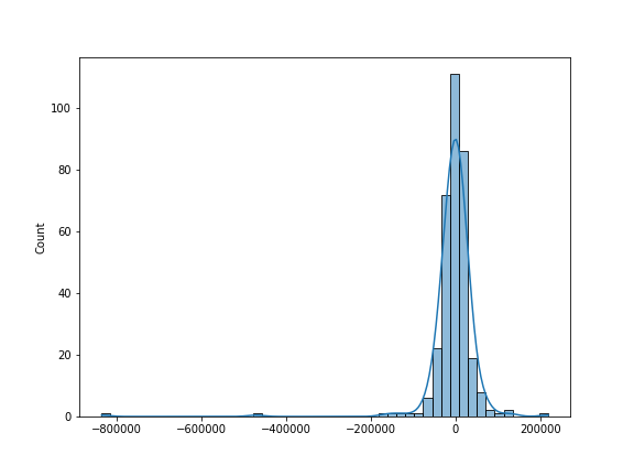
We can also plot the residual:

sns.histplot((y_test-lr_predictions),bins=50,kde=True);

Just to underscore how little we had to do, here's the whole example again, in three lines:

# Initialize the linear regression estimator
lr_model = LinearRegression()

# Fit the model
lr_model.fit(X_train, y_train)

# Generate predictions
lr_predictions = lr_model.predict(X_test)

Performance metrics

Once we've fit our model, it's natural to want to know how well it performs. In machine learning, the focus of model performance is on prediction; typically, we have some objective quantitative metric we care about, and to the degree that a model can produce better values on that metric, we incline to evaluate it more favorably. This doesn't mean that we have to single-mindedly base our evaluation of model on just one quantity; in practice, many other considerations may come into play (e.g., computational efficiency, interpretability, etc.). The point is mainly that machine learning practitioners—at least in applied settings—tend to care much more than traditional scientists do about what models can actually do, and much less about what's going on inside them.

The coefficient of determination

For the rest of this tutorial, we're going to focus our attention on one particular metric of predictive performance: the coefficient of determination, or \(R^2\). \(R^2\) quantifies the proportion of variance in the outcome variable (e.g., house price) explained by the fitted model:

R-squared (R2) is the measure used to determine which line minimizes this distance:

\(R^2\) is the most widely used measure of performance in the individual differences literature, and we'll stick with tradition here. But this shouldn't be taken as an indication that there's anything particularly special about \(R^2\). In fact, in many applications, it's a pretty bad metric, because it's defined with reference to the relative variation in a particular sample, and completely ignores the absolute deviation of predictions from the true scores (i.e., a model can have an \(R^2\) of 1 while generating a predicted score distribution entirely outside the range of the true scores). For our purposes though, \(R^2\) is a sensible metric, because for most individual differences variables, absolute scores don't really mean anything anyway—we're almost always interested in how variation across individuals relates to variation in some other measure or construct.

Here are three other common evaluation metrics for machine learning problems:

• Mean Absolute Error (MAE) is the mean of the absolute value of the errors:

\[\frac 1n\sum_{i=1}^n|y_i-\hat{y}_i|\]

• Mean Squared Error (MSE) is the mean of the squared errors:

\[\frac 1n\sum_{i=1}^n(y_i-\hat{y}_i)^2\]

• Root Mean Squared Error (RMSE) is the square root of the mean of the squared errors:

\[\sqrt{\frac 1n\sum_{i=1}^n(y_i-\hat{y}_i)^2}\]

Comparing these metrics:

• MAE is the easiest to understand, because it's the average error.
• MSE is more popular than MAE, because MSE "punishes" larger errors, which tends to be useful in the real world.
• RMSE is even more popular than MSE, because RMSE is interpretable in the "y" units.

All of these are loss functions, because we want to minimize them.

How well did we do?

Let's see how well the linear regression model we fitted earlier (using the house features as predictors) explains the variance in sales price. We'll make use of scikit-learn's metrics module, which contains a large number of predefined performance metrics. As is true of Estimator objects, all metrics in scikit-learn follow the same usage pattern: we pass in the true scores and the model's predicted scores, respectively.

# the metrics module contains predefined scoring functions
# for commonly used metrics like r^2, MSE, etc. 
from sklearn import metrics

# scoring functions are called by passing an array of
# true scores and and an array of predicted scores as
# inputs
print('Model score:', metrics.r2_score(y_test, lr_predictions))
print('MAE:', metrics.mean_absolute_error(y_test, lr_predictions))
print('MSE:', metrics.mean_squared_error(y_test, lr_predictions))
print('RMSE:', np.sqrt(metrics.mean_squared_error(y_test, lr_predictions)))

Model score: 0.5238801531365112
MAE: 26110.712069211004
MSE: 3851956330.37256
RMSE: 62064.130787215254

Looking at the \(R^2\) score we get the amount of variance explained by the model, which means we can explain about 52% of the variance in sales price using 27 features of the home.

For convenience, scikit-learn estimators have a .score() method you can use as an alternative to the above. Instead of generating predicted scores and then explicitly feeding them to a metric function like r2_score, you can call .score() directly on the estimator after the fit() step, and the prediction will be done implicitly:

# Initialize the estimator and fit the data, just like before
lr_model = LinearRegression()
lr_model.fit(X_train, y_train)
# Now instead of generating predictions explicitly,
# we just call .score(). Note that we lose the ability to
# specify the metric: LinearRegression.score() always uses
# the R^2 metric.
lr_model.score(X_test, y_test)

0.5238801531365112

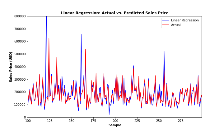
We can also look at how well we did visually by plotting the predicted vs. actual sales price values:

range_plot = range(100,300)

fig, ax = plt.subplots(figsize=(10,6))
lr_1 = ax.plot(range_plot, lr_predictions[range_plot], color='blue', label='Linear Regression')
lr_2 = ax.plot(range_plot, y_test[range_plot], color='red', label = 'Actual')
ax.set_ylim(0, 800000)
ax.set_xlim(range_plot[0], range_plot[-1])
plt.title('Linear Regression: Actual vs. Predicted Sales Price', fontweight='bold')
plt.xlabel('Sample', fontweight='bold')
plt.ylabel('Sales Price (USD)', fontweight='bold')
plt.legend(handles=[lr_1[0],lr_2[0]])
plt.show()